At its heart, Mathematica has deep support for functional programming. As a computer algebra system, the functional programming support in Mathematica is unmatched in similar products, specifically, when it comes to pattern matching and rule based programming.
This post is a walk through the differences and similarities between the approaches that can be taken to solve a problem using both Scala and Mathematica, with a focus on the expressiveness and fluency of the solution code.
Quick Sort
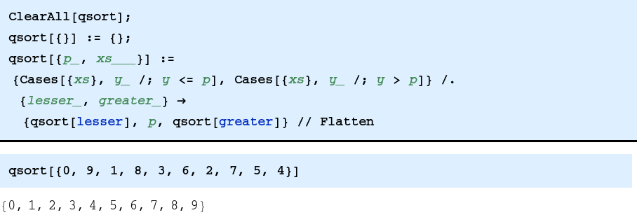
To get into the context, the following is an implementation of the Quick Sort algorithm in Mathematica.
The code demonstrates pattern matching, pattern guards and rule based programming. Cases is the partioning function, while a rule is used to capture the resulting partitions tuple. The qsort function itself is a pattern based function similar to Haskell and Alice style of function definitions.
The Scala implementation uses the partition method to split the list around the pivot p
def qsort[T <% Ordered[T]](list: List[T]): List[T] = list match {
      case Nil     => Nil
      case p :: xs =>
        val (lesser, greater) = xs partition (_ <= p)
        qsort(lesser) ++ List(p) ++ qsort(greater)
    }
Another Scala version could have been implemented using list comprehension, which is much similar to the Mathematica one:
def qsort2[T <% Ordered[T]](list: List[T]): List[T] = list match {
      case Nil     => Nil
      case p :: xs =>
        qsort2(for(x <- xs if x <= p) yield x) ++
        List(p) ++
        qsort2(for(x <- xs if x > p) yield x)
    }
Power Set
A Power set is one of Neat Examples that demonstrates the power of Mathematica’s Fold higher-order function.
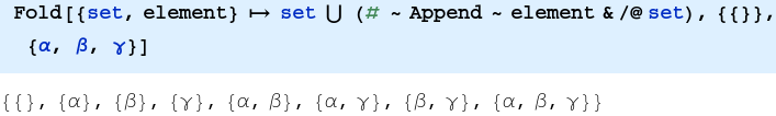
The Scala implementation as almost as expressive, in fact, you might find it more readable and easier to understand.
def powerSet[A](s: Set[A]) =
    s.foldLeft(Set(Set.empty[A])) {
      (set, element) =>
        set union (set map (_ + element))
    }
Here is a example of this implementation in action:
val ps = powerSet(Set('α', 'β', 'γ'))
    println(ps.asString)
Which will result into
[[],[α],[α,γ],[γ],[α,β,γ],[β],[β,γ],[α,β]]
Mathematica Cases
The Cases function in Mathematica can be used to perform filtering based on pattern matching, for example:
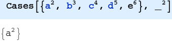
is used to select those expressions in the form of base and exponent, only when the exponent is equal to the constant 2 regardless of the base. Because Mathematica is a symbolic language, the mathematical expressions are first class constructs, and Mathematica is designed to perform operations on such expressions. This is obviously not what we are trying to compare, so we need to define the ADT Power:
case class Power(val base: Symbol, val exp: Int)
In this case, the Scala equivalent is pretty straight forward,
val l = Power('a, 2) :: Power('b, 3) :: Power('c, 4) :: Nil


    val cases0 =
    l flatMap {
      case p@Power(_, 2) => Some(p)
      case _ => None
    }
Taking this a little bit further, the following code tries to match any expression provided that the exponent is even, notice the /; before the predicate EvenQ
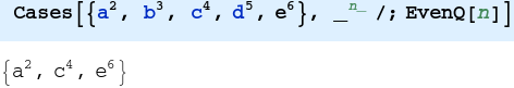
Still, pretty simple in Scala:
l flatMap {
      case p@Power(_, n) if n % 2 == 0 => Some(p)
      case _ => None
    }
One interesting feature of the Cases function, is that it allows direct transformation of matched elements, for example:
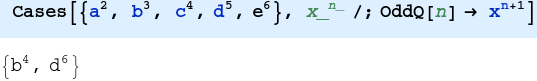
Here, the pattern matches terms with odd exponent, and transforms them into even ones by adding 1 to the exponent. Again, the Scala equivalent is not that hard to implement or less expressive:
l flatMap {
      case p@Power(x, n) if n % 2 != 0 => Some(Power(x, n + 1))
      case _ => None
    }
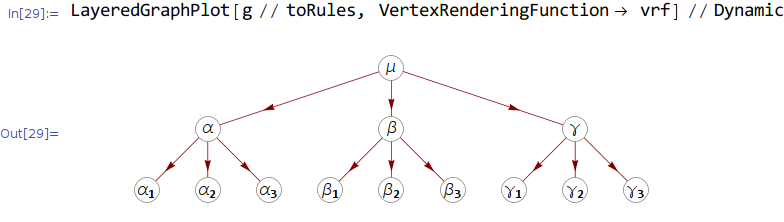
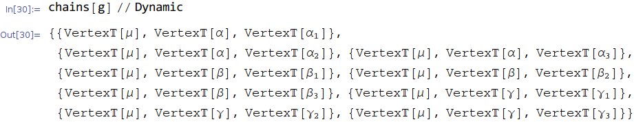
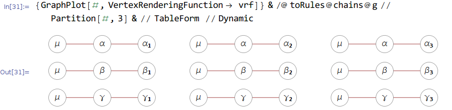
NestWhileList
NestWhileList is one of the powerful and commonly used higher-order function in Mathematica.
Here is a simple example of the function:
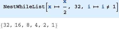
Starting with an intial value 32, NestWhileList nests the application of the actual argument pure function, reporting the result of each application as a list, and terminating when the argument predicate returns true.
This is basically what a Stream in Scala is designed to do, but without the termination, so, a simple implementation of NestWhileList in Scala can look like the following:
def nestWhileList[A](f: A => A, initial: A, p: A => Boolean) = {
    val result = Stream.iterate(initial)(f).takeWhile(p).toList
    result :+ f(result.last)
  }
An equivalent call to the Mathematica call might look like this:
nestWhileList((_: Int) / 2, 32, (_: Int) != 1)
Now consider the definition of the this function:
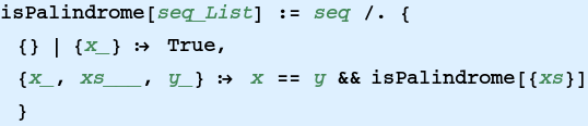
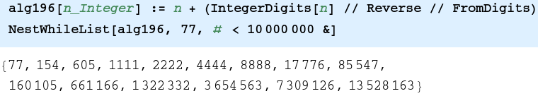
The function checks if a list is palindrome. An algorithm known as Algorithm 196 that generates palindromes can be defined by:
Which can be expressed in Scala as:
val alg196 = (n: Int) => n + n.toString.reverse.toInt

  @tailrec
  def isPalindrome[A <% Ordered[A]](a: List[A]): Boolean = a match {
    case Nil | _ :: Nil => true
    case x :: xs        => x == xs.last && isPalindrome(xs.init)
  }
To generate a list of palindromes in Mathematica, one could write:
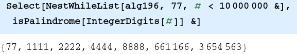
Which can similarly be done in Scala as:
nestWhileList(alg196, 77, (_: Int) < 10000000).
       filter (n => isPalindrome(n.toString.toList))
More examples on the usage of NextWhileList follows.
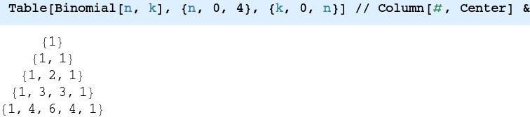
Pascal Triangle
In Mathematica, the Pascal Triangle can be defined by:
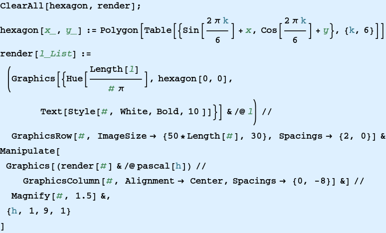
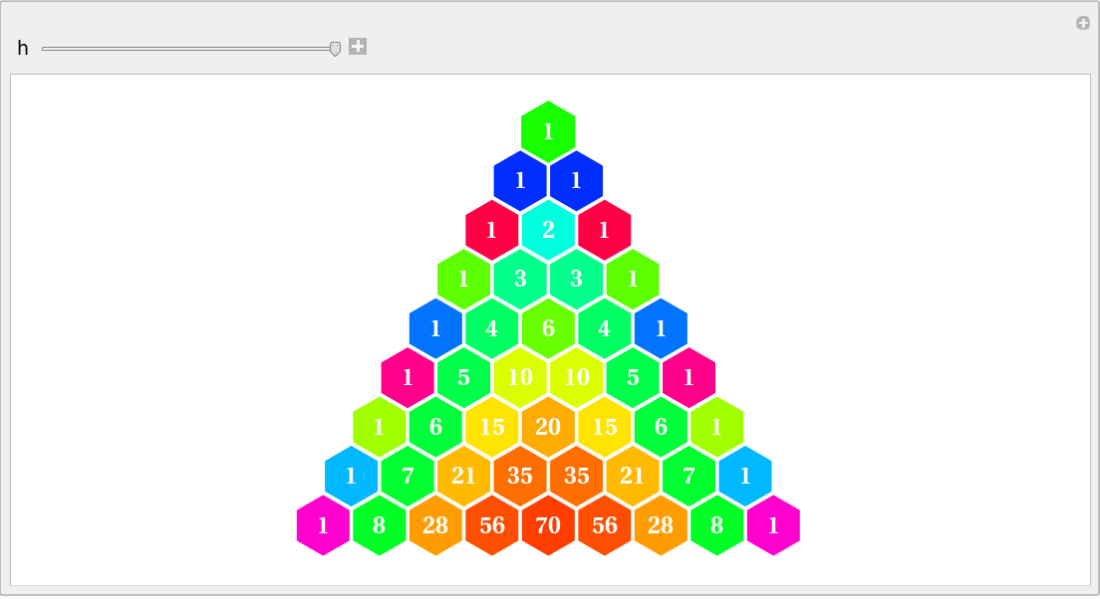
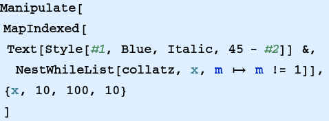
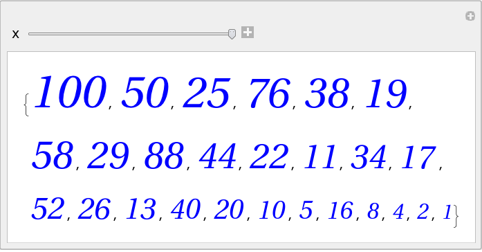
But let’s define it in the naive way, assuming we have no idea what a binomial is, notice what the combination of the tuples and NestWhileList functions will result into:
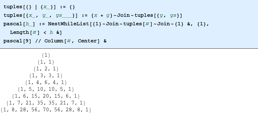
Which forms a model for a nice manipulation
The implementation in Scala is almost identical, concerning both our tuples and pascalTriangle functions:
def pascalTriangle(n: Int) = {

    def tuple(l: List[Int]): List[Int] = l match {
      case Nil | _ :: Nil  => Nil
      case x :: y :: ys    => (x + y) :: tuple(y :: ys)
    }

    nestWhileList[List[Int]](l => (1 :: tuple(l)) :+ 1, List(1), _.length < n)
  }
3N+1 Problem
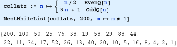
There are several ways to play with the Collatz conjecture in Mathematica, the following is the definition in terms of a piecewise function:
Again, the Scala implementation is as expressive:
def collatz(n: Int) = n match {
    case n if n % 2 == 0  => n / 2
    case n                => (3 * n) + 1
  }
val cs = nestWhileList(collatz(_: Int), 200, (_: Int) != 1)
    println(cs.asString)
[200,100,50,25,76,38,19,58,29,88,44,22,11,34,17,52,26,13,40,20,10,5,16,8,4,2,1]
There is a nice thread here if you would like to see different solutions to this problem in several programming languages.
Bubble Sort
Orginal code of this bubble sort implementation is posted here
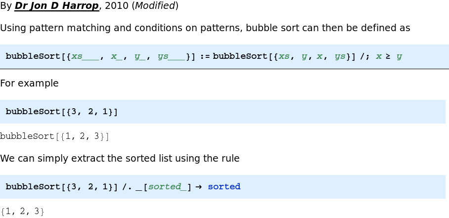
The problem with this Mathematica implementation is that Scala cannot do pattern matching involving arbitrary length prefix, to do this we need to define our version of suffix match method:
The suffixMatch method
@tailrec
  def suffixMatch[A, B](l: List[A], prefix: List[A] = Nil)
                       (f: PartialFunction[List[A], B]): Option[(List[A], B)] =
    l match {
      case Nil                    => None
      case xs if f isDefinedAt xs => Some((prefix, f(xs)))
      case x :: xs                => suffixMatch(xs, prefix :+ x)(f)
    }
The method tries to match the suffix of a list by recursively invoking an argument matching function, dropping the prefix on each iteration. If the function succeeds, the suffixMatch method returns both the dropped prefix and the matched suffix.
We can then define a nice version of this function, to be used more naturaly as the match keyword:
implicit def matchOps[A](l: List[A]) = new {
    def smatch[B](f: PartialFunction[List[A], B], prefix: List[A] = Nil) =
      suffixMatch(l, prefix)(f)
  }
Bubble Sort in Scala
A typical translation of the Mathematica version can then be expressed in Scala this way:
@tailrec
  def bubbleSort(l: List[Int]): List[Int] = {
    l smatch {
      case x :: y :: ys if x > y => y :: x :: ys
    } match {
      case None         => l
      case Some((p, s)) => bubbleSort(p ++ s)
    }
  }
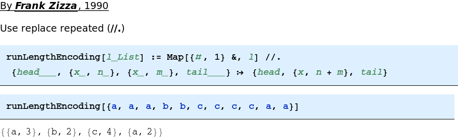
Run Length Encoding
An amazing, famous run length encoding implementation in Mathematica is:
Using our new smatch method, the implementation can be ported to Scala, almost as is:
@tailrec
  def runLengthEncoding[A](l: List[(A, Int)]): List[(A, Int)] = {
    l smatch {
      case (x1, n) :: (x2, m) :: ys if x1 == x2 => (x1, (m + n)) :: ys
    } match {
      case None         => l
      case Some((p, s)) => runLengthEncoding(p ++ s)
    }
  }
Conclusion
Scala is an amazingly expressive and, more importantly, beautiful language. The design and implementation of the core idea of expanding the library not the language, makes Scala a extremely powerful and expressive tool for modeling solutions to simple and complex problems alike.